Non-commutative algebras,
computer algebra systems,
and theorem provers
Eric Wieser
formerly: Cambridge University Engineering Department slides: eric-wieser.github.io/brown-2024/seminar 2024-12-04Non-commutative algebras
Non-commutative algebras Geometric motivation
Geometry is inherently non-commutative:
- applying 3D rotations in a different order gives a different result
- the oriented plane spanning $u$ and $v$ faces the opposite way to the one spanning $v$ and $u$
… algebraic representations of geometry are too:
- for rotation matrices, composition is multiplication, and $R_1R_2 \ne R_2R_1$ in general
- the normal vector of such a plane (in 3D) can be found with the cross product, and $u\times v = -v\times u$.
The matrix algebra $\mathbb{R}^{n \times n}$ is the typical choice for representing geometry, but is by no means the only choice available:
Quaternions
$\mathbb{H}$
Exterior algebra
$\bigwedge(V)$
Geometric algebra
$\mathcal{G}(Q)$
Non-commutative algebras Geometric examples
Quaternions, $\mathbb{H}$
Like the complex numbers, $q = r + x\mathrm{i} + y\mathrm{j} + z\mathrm{k}$, but with $i^2 = j^2 = k^2 = ijk = −1$.
In 3D, a rotation around the axis $u$ by $\theta$ can be represented as:
$$e^{\frac{\theta}{2}{(u_x\mathrm{i} + u_y\mathrm{j} + u_z\mathrm{k})}} = \cos \frac{\theta}{2} + (u_x\mathrm{i} + u_y\mathrm{j} + u_z\mathrm{k}) \sin \frac{\theta}{2}$$Applying a quaternion rotation is done as $qvq^{-1}$.
Every (normed) quaternion represents a rotation; typically a better choice than rotation matrices which can become non-orthonormal.
A division ring, unlike the matrix algebra; all non-zero quaternions have an inverse.
Exterior algebra, $\bigwedge(V)$
Geometric algebra, $\mathcal{G}(Q)$
Non-commutative algebras Geometric examples
Quaternions, $\mathbb{H}$
Exterior algebra, $\bigwedge(V)$
For an arbitrary vector space $V$ containing $u, v$, $$u \wedge v = -v \wedge u$$ represents an oriented plane at the origin spanning $u$ then $v$.
Unlike the cross product, generalizes to higher dimensions: $u \wedge v \wedge w$ is an oriented volume.
Geometric algebra, $\mathcal{G}(Q)$
An extension of exterior algebra that includes a metric $Q$, which results in a dot product $u \cdot v$. Multiplication of vectors satisfies:
$$\begin{align*} uv &= u\cdot v + u \wedge v \\ \implies uv &= vu - 2u\cdot v \end{align*}$$Non-commutative algebrasWeaker algebraic structures
- $ab \ne ba$; non-commutativity
-
As we saw, this is particularly easy to motivate through geometry. This paves the way to further
weakening
of our algebraic rules. - $a \ne 0, b \ne 0, ab = 0$; zero divisors
-
$\mathbb{R}^{n \times n}$ and $\bigwedge(B)$ and $\mathcal{G}(Q)$ all have this property.
This means $ab = ac \nRightarrow b = c$ even if $a \ne 0$!
- $a(bc) \ne (ab)c$; non-associativity
-
A simple example is the vector cross product:
$$u \times (v \times w) = (u \times v) \times w + v \times (u \times w)$$More examples: Lie algebras, Octonions, …
Forgetting these weaknesses leads to algebraic mistakes.
Can we software help us keep track of them?
Computer algebra systems
A computer algebra system (CAS) or symbolic algebra system (SAS) is any mathematical software with the ability to manipulate mathematical expressions in a way similar to the traditional manual computations of mathematicians and scientists.Computer algebra system Wikipedia
Useful for
- Roughly checking your work
- Answering what-if questions experimentally
- Solving large but tedious equations quickly
- …
Typical features
- Algebraic simplification
- Root finding
- Integration and differentiation
- Arbitrary precision calculations
- …
Notable implementations
(1965, BSD)
(1982, GPL)
(1982, Proprietary)
(1993, Proprietary)
(1998, Proprietary)
(2004, GPL)
Sympy
SymPy is a Python library for symbolic mathematics. It aims to become a full-featured computer algebra system (CAS) while keeping the code as simple as possible in order to be comprehensible and easily extensible. SymPy is written entirely in Python.
Why wasn't this on the previous slide?
Sage[Math] tries to gather together all the major open source mathematics software, and glue it together into a useful system. In fact, Sage[Math] includes SymPy as one of its systems.
What is the difference between SymPy and Sage[Math]? Aaron Meurer (Lead SymPy developer)
Sympy Examples
Solve $x^2 - 2 = 0$
                >>> solve(x**2 - 2, x)
                $\left[ - \sqrt{2}, \  \sqrt{2}\right]$
Take the derivative of $\sin{(x)}e^x$
                >>> diff(sin(x)*exp(x), x)
                $e^{x} \sin{\left(x \right)} + e^{x} \cos{\left(x \right)}$
Compute $\int_{-\infty}^\infty \sin{(x^2)}\,dx$
                >>> integrate(exp(x)*sin(x) + exp(x)*cos(x), x)
                $e^{x} \sin{\left(x \right)}$
Solve the differential equation $y'' - y = e^t$
                  >>> y = Function('y')
                  >>> dsolve(Eq(y(t).diff(t, t) - y(t), exp(t)), y(t))
                  $y{\left(t \right)} = C_{2} e^{- t} + \left(C_{1} + \frac{t}{2}\right) e^{t}$
The Power of Symbolic Computation SymPy.org
SympyExpression trees
>>> from sympy import *; from this_presentation import show_repr
Real numbers
              >>> x, y = symbols('x y', real=True)
              >>> expr = (x + y)*(x - y); expr
              $(x - y)(x + y)$
              >>> show_repr(expr)
              Mul(Add($x$, Mul(Integer(-1), $y$)),
                  Add($x$, $y$))
Complex numbers
              >>> x, y = symbols('x y', complex=True)
              >>> expr = (x + y)*(x - y); expr
              $(x - y)(x + y)$
              >>> show_repr(expr)
              Mul(Add($x$, Mul(Integer(-1), $y$)),
                  Add($x$, $y$))
Underlying representations
- Real
Symbol,Add,Mul, …- Complex
Symbol,Add,Mul, …- Matrix
MatrixSymbol,MatAdd,MatMul, …- Quaternions?
Matrices
              >>> m, n = symbols('m n')
              >>> X = MatrixSymbol('X', m, n)
              >>> Y = MatrixSymbol('Y', m, n)
              >>> expr = (X + Y)*(X - Y).T; expr
              $(X + Y)(X^T - Y^T)$
              >>> show_repr(expr)
              MatMul(
                  MatAdd($X$, $Y$),
                  MatAdd(
                      Transpose($X$),
                      MatMul(Integer(-1), Transpose($Y$))))
SympyExpression trees
Quaternions
No symbolic quaternions; only quaternions with symbolic coefficients.
            >>> x, xi, xj, xk = symbols('x x_i x_j x_k');  xq = Quaternion(x, xi, xj, xk)
            >>> y, yi, yj, yk = symbols('y y_i y_j y_k');  yq = Quaternion(y, yi, yj, yk)
            >>> expr = xq * yq; expr
            $\left(x y - x_{i} y_{i} - x_{j} y_{j} - x_{k} y_{k}\right) + \left(x y_{i} + x_{i} y + x_{j} y_{k} - x_{k} y_{j}\right) i$
            $\quad+ \left(x y_{j} - x_{i} y_{k} + x_{j} y + x_{k} y_{i}\right) j + \left(x y_{k} + x_{i} y_{j} - x_{j} y_{i} + x_{k} y\right)$
            >>> show_repr(expr)
            Quaternion(Add(Mul($x$, $y$), Mul(Integer(-1), $x_i$, $y_i$), Mul(Integer(-1), $x_j$, $y_j$), Mul(Integer(-1), $x_k$, $y_k$)),
                       Add(Mul($x$, $y_i$), Mul($x_i$, $y$), Mul($x_j$, $y_k$), Mul(Integer(-1), $x_k$, $y_j$)),
                       Add(Mul($x$, $y_j$), Mul(Integer(-1), $x_i$, $y_k$), Mul($x_j$, $y$), Mul($x_k$, $y_i$)),
                       Add(Mul($x$, $y_k$), Mul($x_i$, $y_j$), Mul(Integer(-1), $x_j$, $y_i$), Mul($x_k$, $y$)))
This makes quaternions hard to work with:
$x_qx_qx_q^{-1}y_q = x_qy_q$
              >>> (xq * xq * xq**-1 * yq).simplify()
              $\left(x y - x_{i} y_{i} - x_{j} y_{j} - x_{k} y_{k}\right) + \left(x y_{i} + x_{i} y + x_{j} y_{k} - x_{k} y_{j}\right) i$
              $\qquad + \left(x y_{j} - x_{i} y_{k} + x_{j} y + x_{k} y_{i}\right) j + \left(x y_{k} + x_{i} y_{j} - x_{j} y_{i} + x_{k} y\right) k$
$\nabla_{\!x_q}(x_qy_q) = -2y_q$
              >>> def q_diff(Φ, dq):  # similar to ∇Φ
              ...     ℍ = Quaternion
              ...     I, J, K = ℍ(0,1,0,0), ℍ(0,0,1,0), ℍ(0,0,0,1)
              ...     return (Φ.diff(dq.a) + I*Φ.diff(dq.b)
              ...         + J*Φ.diff(dq.c) + K*Φ.diff(dq.d))
              >>> q_diff(xq*yq, xq)
              $- 2 y + - 2 y_{i} i + - 2 y_{j} j + - 2 y_{k} k$
SympyExamples with matrix determinants
>>> m, n = symbols('m, n')
              >>> A = MatrixSymbol('A', n, n)
              >>> B = MatrixSymbol('B', n, n)
              >>> P = MatrixSymbol('P', m, n)
              >>> Q = MatrixSymbol('Q', n, m)
              >>> Eq(det(A*B), det(A)*det(B))
              $\text{True}$
Eq can be used to write down a symbolic equality.
MatMul._eval_determinant is expanding the determinant for us.
              >>> Eq(det(A*B*A.inv()), det(B))
              $\left|{A^{-1}}\right| \left|{A}\right| \left|{B}\right| = \left|{B}\right|$
              >>> Eq(det(A*B*A.inv()), det(B)).simplify()
              $\text{True}$
_eval_determinant gets us partway there, but doesn't finish the job.
simplify() can clean up.
Weinstein–Aronszajnidentity)
>>> I = Identity >>> Eq(det(I(m) + P*Q), det(I(n) + Q*P)) $\left|{\mathbb{I} + PQ}\right| = \left|{\mathbb{I} + QP}\right|$ >>> Eq(det(I(m) + P*Q), ... det(I(n) + Q*P)).simplify() NonSquareMatrixError: Det of a non-square matrix>>> I = Identity >>> Eq(det(I(n) + A*B), det(I(n) + B*A)) $\left|{\mathbb{I} + AB}\right| = \left|{\mathbb{I} + BA}\right|$ >>> Eq(det(I(n) + A*B), ... det(I(n) + B*A)).simplify() AttributeError: 'Mul' object has no attribute 'shape'
There is no MatAdd._eval_determinant to help here.
simplify() is ad-hoc, and can crash! Switching to square matrices makes things worse!
SympyWhat's going wrong?
Consider supporting a new algebra, MyAlg. We have two big hurdles:
Expression tree extension
It looks like we have to build new MyAlgAdd, MyAlgMul, … objects.
This scales poorly if we want to work with things like matrices of MyAlg; do we need MatMyAlgAdd e.t.c.?
If we get this wrong, things like simplify() fail if they expect MyAlgMul but get a Mul.
Supporting symbols
Defining our objects as structures with fields like we would in a conventional programming language isn't enough.
Expression tree objects needs to know how to simplify themselves.
This local simplification doesn't scale to things like $$\operatorname{det}(1 + AB) = \operatorname{det}(1 + BA).$$
Are we sure our simplifications are mathematically sound?
What if our programming language could handle all of this?
Theorem provers
A proof assistant [or theorem prover] is a piece of software that provides a language for defining objects, specifying properties of these objects, and proving that these specifications hold. The system checks that these proofs are correct down to their logical foundation.
These tools are often used to verify the correctness of programs. But they can also be used for abstract mathematics [...]. In a formalization, all definitions are precisely specified and all proofs are virtually guaranteed to be correct.
What is a proof assistant? Lean community website
Theorem proversNotable implementations
- About a decade less mature than computer algebra systems (gray)
- Mizar (1973), Isabelle (1986), HOL Family (1988)
- Coq (1989), Metamath (1993), Agda (2007)
- Lean 1 (2013), Lean 2 (2015), & Lean 3 (2016)
Lean had the advantage of being born later and learning from past mistakes.
CICM 2020 slack Mario Carneiro, Lean Maintainer
- Lean 4 (2023)
- Actively developed by the Lean Focused Research Organization
- Can be used in-browser or in supported IDEs: VS Code and Emacs
- Better support for domain-specific syntax and custom automation
- Native code and its formal verification in one language
Theorem proversDifferences with computer algebra systems
Computer algebra systems
Easier and faster to use
More of a focus of algorithms to solve specific problems
Sometimes tricky to extend
No strong guarantees of correctness
Theorem provers
Steeper learning curve
Focus on correctness; very small core
which requires trust.
Very extensible, as even things like equality, =, are built as extensions to the core!
Lean in Practice
Lean in Practice Definitions, Types, and Terms
            -- name : type := value (or "term")
            def two : ℕ := 2

            def double (a : ℕ) : ℕ := two * a

            -- syntax for `Exists fun x : ℕ ↦ Eq (double x) 3`
            def Unlikely : Prop := ∃ x : ℕ, double x = 3
            lemma unlikely_proof : unlikely := sorry

            lemma double_is_add_self (a : ℕ) : double a = a + a := by
              dsimp [double, two]
              apply two_mul
ℕ = Nat.
mathematicians [have] lower tolerance for unintuitive interfaces than computer scientists.
CICM 2020 slack Mario Carneiro, PhD in Logic, Lean Maintainer
double is function that takes and outputs a ℕ.
It has type ℕ → ℕ.
A Prop is a mathematical statement.
Behind this nice syntax lies an expression tree
Prop instances are themselves Types.
Values are their proofs.
Note that a is analogous to a sympy.Symbol here
Arguments to functions and symbols in mathematical statements are the same thing!
double_is_add_self 1 is a proof that double 1 = 1 + 1
dsimp and apply are tactics,
to help us construct proofs interactively.
two_mul is a lemma from the library.
Lean in Practice class for abstraction
class for abstraction
            class AddCommGroup (A : Type)
              extends Add A, Zero A, Neg A : Type where
            add_comm       : ∀ a b : A,         a + b = b + a
            add_assoc      : ∀ a b c : A, (a + b) + c = a + (b + c)
            zero_add       : ∀ a : A,           0 + a = a
            add_one        : ∀ a : A,           a + 0 = a
            neg_add_cancel : ∀ a : A,          -a + a = 0
AddCommGroup is the name of our type-class.
A makes this a dependent type,
AddCommGroup A is a collection of proofs that A forms an abelian group.
extends is inheritance.
Used here to provide +, 0 and - for A.
Theorems consume the API so as to generalize to all abelian groups...
                  lemma neg_add {A : Type} [AddCommGroup A] (a b : A) :
                    -(a + b) = -a + -b := sorry
$\mathbb{H}$ and $\mathbb{R}^{m\times n}$ implement the API to prove they are abelian:
                    instance : AddCommGroup ℍ where
                      add_assoc := sorry; add_comm := sorry
                      zero_add := sorry;  add_zero := sorry
                      neg_add_cancel := sorry
                    instance : AddCommGroup (matrix m n ℝ) where
                      add_assoc := sorry; add_comm := sorry
                      zero_add := sorry;  add_zero := sorry
                      neg_add_cancel := sorry
Lean in PracticeExpression Trees
Lean is hiding a much more complex expression tree than sympy:
            variable {x y : ℝ}
            #show_repr x + y -- custom command for these slides
            app
              (app
                (app
                  (app
                    (app
                      (app (const `HAdd.hAdd [Level.zero, Level.zero, Level.zero]) (const `Real []))
                      (const `Real []))
                    (const `Real []))
                  (app (app (const `instHAdd [Level.zero]) (const `Real [])) (const `Real.instAdd [])))
                (fvar { name := `x }))
              (fvar { name := `y })
but we usually want it to remain hidden:
                  set_option pp.all true
                  #check x + y
                  @HAdd.hAdd.{0, 0, 0} Real Real Real
                    (@instHAdd.{0} Real Real.instAdd) x y
                  #check x + y
                  x + y
Key difference from sympy - the expression tree:
- uses
fvarfor all symbol types - is used by the language itself!
Lean in PracticeExamples with matrix determinants
            import Mathlib.LinearAlgebra.Matrix.SchurComplement
            variable {R m n : Type} [CommRing R] [Fintype m] [Fintype n] [DecidableEq m] [DecidableEq n]
            variable (A B : Matrix n n R) (P : Matrix m n R) (Q : Matrix n m R)
            open Matrix         -- for `det`
              example :
                  det (A*B) = det A * det B := by
                simp
* is matrix multiply.
example : det (A*B*A⁻¹) = det B := sorryexample (hA : IsUnit A) : det (A*B*A⁻¹) = det B := sorryexample (hA : IsUnit A) : det (A*B*A⁻¹) = det B := by simp [hA]⊢ A.det * B.det * Ring.inverse A.det = B.detexample (hA : IsUnit A) : det (A*B*A⁻¹) = det B := by exact?Try this: exact det_conj hA Bexample (hA : IsUnit A) : det (A*B*A⁻¹) = det B := by exact det_conj hA B
We need a proof that A is invertible, spelt IsUnit A.
simp takes us to a dead end.
exact? finds the proof.
              example :
                  det (1 + P*Q) = det (1 + Q*P) := by
                simp⊢ (1 + P * Q).det = (1 + Q * P).det
Lean doesn't know this result yet; let's prove it!
Lean in PracticeProving the Weinstein–Aronszajn identity
How do we prove $\operatorname{det} (1 + PQ) = \operatorname{det} (1 + QP)$ by hand?
                /-- The Weinstein–Aronszajn identity -/
                lemma Matrix.det_one_plus_comm :
                    det (1 + P*Q) = det (1 + Q*P) := by
                  calc det (1 + P*Q) = det (fromBlocks 1 (-P) Q 1) := ?_
                    _                = det (1 + Q*P)               := ?_
                  · rewrite [det_fromBlocks_one₂₂]
                    rewrite [Matrix.neg_mul]
                    rewrite [sub_neg_eq_add]
                    rfl
                  · rw [det_fromBlocks_one₁₁, Matrix.mul_neg,
                        sub_neg_eq_add]
R : Type m : Type n : Type inst✝⁴ : CommRing R inst✝³ : Fintype m inst✝² : Fintype n inst✝¹ : DecidableEq m inst✝ : DecidableEq n P : Matrix m n R Q : Matrix n m R ⊢ det (1 + P*Q) = det (1 + Q*P)P : Matrix m n R Q : Matrix n m R ⊢ det (1 + P*Q) = det (1 + Q*P)P : Matrix m n R Q : Matrix n m R ⊢ det (1 + P*Q) = det (fromBlocks 1 (-P) Q 1) P : Matrix m n R Q : Matrix n m R ⊢ det (fromBlocks 1 (-P) Q 1) = det (1 + Q*P)P : Matrix m n R Q : Matrix n m R ⊢ det (1 + P*Q) = det (fromBlocks 1 (-P) Q 1)P : Matrix m n R Q : Matrix n m R ⊢ det (1 + P*Q) = det (1 - -P*Q)P : Matrix m n R Q : Matrix n m R ⊢ det (1 + P*Q) = det (1 - -(P*Q))P : Matrix m n R Q : Matrix n m R ⊢ det (1 + P*Q) = det (1 + P*Q)goals accomplished 🎉⊢ det (fromBlocks 1 (-P) Q 1) = det (1 + Q*P)goals accomplished 🎉
Lean provides the goal view, reminding us what we know. Most of the goal view is noise, so let's cut to the signal Outline the proof using the
calc tactic.Each
?_ is a hole, leaving us with two goals (⊢).
We can use · to focus on just the first goal.
Let's expand det (fromBlocks ...) around the bottom right, ...
… push the negation outside the product, …
… and cancel the negations.
We're done!
Now we can go back to the other goal. We can solve it the same way, …
… but let's write it more concisely.
How did Lean know det_fromBlocks_one₁₁ and det_fromBlocks_one₂₂?.
Mathlib
Mathlib
A mathematical library for Lean, comparable to:
- Coq's
mathematical components
- Isabelle's
HOL-Analysis
Curated by a diverse set of over 350 maintainers and contributors:
- role: Professors, Post-docs, PhD students, Undergrads
- origin: USA, France, The Netherlands, UK, Canada, Australia, …
- expertise: Mathematics, Computer Science, Physics, AI, …

What does Mathlib know?
What does Mathlib know?Pythagorean theorem
For a right triangle with legs $a$ and $b$ and hypotenuse $c$,
$$a^2+b^2=c^2.$$
Pythagorean theorem, if-and-only-if angle-at-point form.
                lemma dist_sq_eq_dist_sq_add_dist_sq_iff_angle_eq_pi_div_two
                    {V P : Type*}
                    [NormedAddCommGroup V] [InnerProductSpace ℝ V]
                    [MetricSpace P] [NormedAddTorsor V P]
                    (X Y Z : P) :
                    dist X Z ^ 2 = dist X Y ^ 2 + dist Z Y ^ 2 ↔
                      ∠ X Y Z = π / 2
Right-angled triangles Mathlib docs
Some translation required!
right triangle↔
∠ X Y Z = π / 2
legs $a$ and $b$↔
dist X Y, dist Y Z
hypotenuse $c$↔
dist X Z
parallel postulate ↔ NormedAddTorsor V P
What does Mathlib know?Parseval's theorem
These amplitudes [$c_n$] can be related to the power content of the signal $g(t)$ over one period
$$\sum_{n=-\infty}^{\infty}|c_n|^2 dt = \frac{1}{T}\int_{0}^{T}|g(t)|^2 dt$$where $g(t) = \sum_{n=-\infty}^{\infty}c_ne^{jn\omega_0t}$
The sum of the squared norms of the Fourier coefficients equals the $L^2$ norm of the function.
                lemma tsum_sq_fourierCoeff
                  {T : ℝ} [hT : Fact (0 < T)]
                  (g : Lp ℂ 2 (@haarAddCircle T hT)) :
                  ∑' n : ℤ, ∥fourierCoeff g n∥^2
                  = ∫ t : AddCircle T, ∥g t∥^2 ∂haarAddCircle
Fourier analysis on the circle Mathlib docs
one period↔
t : AddCircle T
$c_n$↔
fourierCoeff g n
$\frac{1}{T}dt$↔
∂haarAddCircle
(the measurearound a circle that sums to 1)
$g(t) = \sum \cdots$↔
g : Lp ℂ 2 (@haarAddCircle T hT)
(g is a function of type AddCircle T → ℂ, with finite $L^2$ norm)
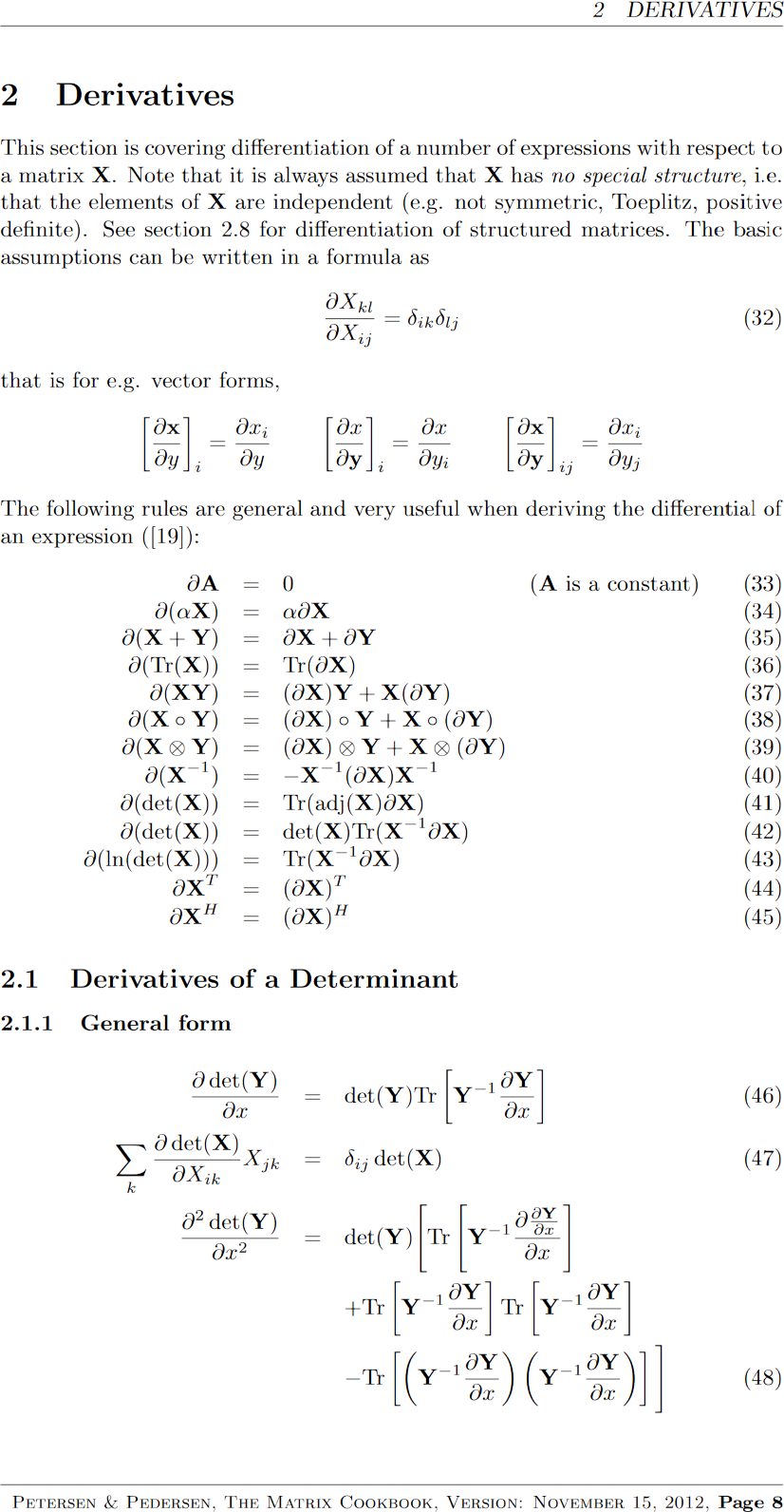
What does Mathlib know?The Cayley-Hamilton theorem
The characteristic polynomial of $A$ is defined as $$\begin{align*} p_{A}(\lambda)&=\det(\lambda I_{n}-A) \\ \textit{[...]}\quad&=\lambda^{n}+c_{n-1}\lambda^{n-1}+\cdots+c_{1}\lambda+c_{0} \end{align*}$$ One can create an analogous polynomial $p_{A}(A)$ [...]. The Cayley–Hamilton theorem states that $p_A(A) = 0$.
Cayley–Hamilton theorem Wikipedia
The characteristic polynomial of a matrix, applied to the matrix itself, is zero. This holds over any commutative ring.
                lemma Matrix.aeval_self_charpoly
                    {R : Type} [CommRing R]
                    {n : Type} [DecidableEq n] [Fintype n]
                    (A : Matrix n n R) :
                    Polynomial.aeval A A.charpoly = 0
Characteristic polynomials and the Cayley-Hamilton theorem Mathlib docs
$p_A$↔
A.charpoly
$p(A)$↔
Polynomial.aeval A p
Note that by [the] Cayley-Hamilton theorem, $e^{A\tau} = I\alpha_0(\tau) + \cdots + A^{n-1}\alpha_{n-1}$
Mathlib does not yet have this corollary, but it is close…
What does Mathlib know?Half an Undergraduate Mathematics Degree
What does Mathlib know?Some fraction of the Matrix cookbook
?
the Matrix cookbook?
A collection of facts (identities, approximations, inequalities, relations, ...) about matrices and matters relating to them [for] a quick desktop referenceThe Matrix Cookbook (2012) Kaare B. Petersen, Michael S. Pedersen
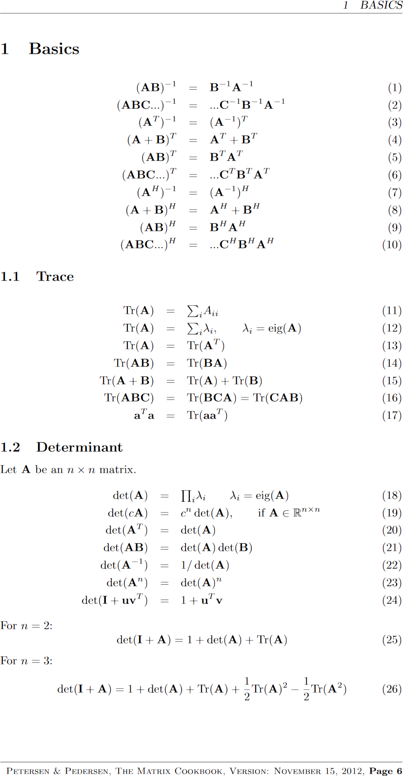
                theorem eq_1 : (A * B)⁻¹ = B⁻¹ * A⁻¹                    := Matrix.mul_inv_rev _ _
                theorem eq_2 :  l.prod⁻¹ = (l.reverse.map Inv.inv).prod := Matrix.list_prod_inv_reverse _
                theorem eq_3 :      Aᵀ⁻¹ = A⁻¹ᵀ                         := (transpose_nonsing_inv _).symm
                theorem eq_4 :  (A + B)ᵀ = Aᵀ + Bᵀ                      := transpose_add _ _
                theorem eq_5 :  (A * B)ᵀ = Bᵀ * Aᵀ                      := transpose_mul _ _
                -- ...
                theorem eq_37 (X : R → Matrix m n R) (Y : R → Matrix n p R)
                              (hX : Differentiable R X) (hY : Differentiable R Y) :
                    (deriv fun a => X a * Y a) = fun a => deriv X a * Y a + X a * deriv Y a :=
                  funext fun a => ((hX a).hasDerivAt.matrix_mul (hY a).hasDerivAt).deriv
HasDerivAt.matrix_mul is not yet in Mathlib!
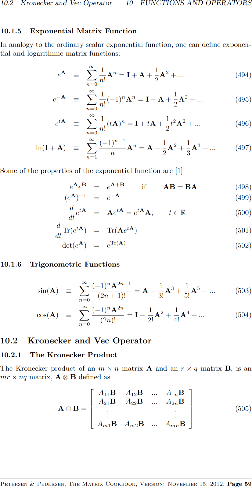
                theorem eq_498 (h : A * B = B * A) : exp ℝ A * exp ℝ B = exp ℝ (A + B) :=
                  (Matrix.exp_add_of_commute _ _ _ h).symm

                theorem eq_499 : (exp ℝ A)⁻¹ = exp ℝ (-A) := (Matrix.exp_neg _ _).symm
22% so far, at eric-wieser/lean-matrix-cookbook

Generalization in Theorem provers
Generalization in Theorem Provers… is just refactoring!
Revisiting the $\exp{A}$ example for matrices:
theorem eq_499 : (exp ℝ A)⁻¹ = exp ℝ (-A) := (Matrix.exp_neg _ _).symm
This didn't always work; exp used to be declared as:
def exp [NontriviallyNormedField 𝕂] [NormedRing 𝔸] [NormedAlgebra 𝕂 𝔸] (x : 𝔸) : 𝔸
leading to an error about no (canonical) norm existing
                theorem eq_499 : (exp ℝ Afailed to synthesize
                  NormedRing (Matrix n n ℝ))⁻¹ = exp ℝ (-A) := sorry
Solution: generalize from normed to topological algebras:
                  def exp
                      [NontriviallyNormedField 𝕂]
                      [NormedRing 𝔸]
                      [NormedAlgebra 𝕂 𝔸]
                      (x : 𝔸) : 𝔸 :=
                    (expSeries 𝕂 𝔸).sum x
                  def exp
                      [Field 𝕂]
                      [Ring 𝔸] [TopologicalSpace 𝔸] [TopologicalRing 𝔸]
                      [Algebra 𝕂 𝔸] [ContinuousConstSMul 𝕂 𝔸]
                      (x : 𝔸) : 𝔸 :=
                    (expSeries 𝕂 𝔸failed to synthesize
                      NontriviallyNormedField 𝕂).sum x
                  def expSeries
                      [NontriviallyNormedField 𝕂]
                      [NormedRing 𝔸]
                      [NormedAlgebra 𝕂 𝔸] :
                      FormalMultilinearSeries 𝕂 𝔸 𝔸 :=
                    fun n => (1/n! : 𝕂) • mkPiAlgebraFin 𝕂 n 𝔸
                  def expSeries
                      [Field 𝕂]
                      [Ring 𝔸] [TopologicalSpace 𝔸] [TopologicalRing 𝔸]
                      [Algebra 𝕂 𝔸] [ContinuousConstSMul 𝕂 𝔸] :
                      FormalMultilinearSeries 𝕂 𝔸 𝔸failed to synthesize
                        NontriviallyNormedField 𝕂 :=
                    fun n => (1/n! : 𝕂) • mkPiAlgebraFin 𝕂 n 𝔸
At each step, Lean tells us what we have to generalize next!
Generalization in Theorem Proversisn't all for free
At each step, Lean tells us what we have to generalize next!
For exp, this is entirely mechanical, but what about deriv,
which also needs matrices to be a normed space?
Lean leads us through deriv → fderiv → HasFDerivAt → HasFDerivAtFilter → IsLittleO, but we're in trouble:
            def IsLittleO [Norm E] [Norm F]
                (l : Filter α) (f : α → E) (g : α → F) : Prop :=
              ∀ ⦃c : ℝ⦄, 0 < c → ∀ᶠ x in l, ‖f x‖ ≤ c * ‖g x‖
We can't have $\|f(x)\|$ without assuming $E$ is normed.
Generalization sometimes requires mathematical insight!
              def IsLittleOTVS
                  [NNNorm 𝕜] [TopologicalSpace E] [TopologicalSpace F]
                  [Zero E] [Zero F] [SMul 𝕜 E] [SMul 𝕜 F]
                  (f : α → E) (g : α → F) (l : Filter α) : Prop :=
                ∀ U ∈ 𝓝 (0 : E), ∃ V ∈ 𝓝 (0 : F), ∀ ε ≠ (0 : ℝ≥0),
                  ∀ᶠ x in l, egauge 𝕜 U (f x) ≤ ε * egauge 𝕜 V (g x)
#9675: define
IsLittleOTVSYury Kudryashov
Generalization in Theorem ProversExamples of definitions
Generalization sometimes requires mathematical insight!
                  def IsLittleO [Norm E] [Norm F]
                      (l : Filter α) (f : α → E) (g : α → F) : Prop :=
                    ∀ ⦃c : ℝ⦄, 0 < c → ∀ᶠ x in l, ‖f x‖ ≤ c * ‖g x‖
                  def IsLittleOTVS
                      [NNNorm 𝕜] [TopologicalSpace E] [TopologicalSpace F]
                      [Zero E] [Zero F] [SMul 𝕜 E] [SMul 𝕜 F]
                      (f : α → E) (g : α → F) (l : Filter α) : Prop :=
                    ∀ U ∈ 𝓝 (0 : E), ∃ V ∈ 𝓝 (0 : F), ∀ ε ≠ (0 : ℝ≥0),
                      ∀ᶠ x in l, egauge 𝕜 U (f x) ≤ ε * egauge 𝕜 V (g x)
(motivation: use deriv on matrices without choosing a norm)
                  def Disjoint
                      [SemilatticeInf α] [OrderBot α]
                      (a b : α) :=
                    a ⊓ b ≤ ⊥
                  def Disjoint
                      [PartialOrder α] [OrderBot α]
                      (a b : α) :=
                    ∀ ⦃x : α⦄, x ≤ a → x ≤ b → x ≤ ⊥
(motivation: a ⊓ b on Finset X needs an algorithm to decide equality on X)
                  structure QuadraticForm
                      [Ring R] [AddCommGroup M] [Module R M] where
                    fn : M → R
                    fn_smul (a : R) (x : M) : fn (a • x) = a * a * fn x
                    polar_add_left' (x x' y : M) :
                      polar fn (x + x') y = polar fn x y + polar fn x' y
                    polar_smul_left' (a : R) (x y : M) :
                      polar fn (a • x) y = a • polar fn x y
                  structure QuadraticForm
                      [CommSemiring R] [AddCommMonoid M] [Module R M] where
                    fn : M → R
                    fn_smul (a : R) (x : M) : fn (a • x) = a * a * fn x
                    exists_companion' :
                      ∃ B : BilinForm R M,
                        ∀ x y, fn (x + y) = fn x + fn y + B x y
(motivation: permits QuadraticForm ℕ ℕ)
Generalization in Theorem ProversAn example of proofs
                  theorem mul_eq_one_comm
                      [CommRing R] [Fintype n] [DecidableEq n]
                      (A B : Matrix n n R) :
                      A * B = 1 ↔ B * A = 1 := by
                    /-
                    argument follows by finding the matrix inverse
                    in terms of the determinant.
                    -/
                  theorem mul_eq_one_comm
                      [CommSemiring R] [Fintype n] [DecidableEq n]
                      (A B : Matrix n n R) :
                      A * B = 1 ↔ B * A = 1 := by
                    /-
                    argument follows through a new `detp` that is only
                    the positive or negative terms in the determinant,
                    and some fiddly handling of additive inverses.
                    -/
(motivation: matrices of natural numbers? Ask the author of the change, Thomas Browning!)
Generalization often comes at the cost of clarity.
What else does Mathlib know?
What else does Mathlib know?The algebra that I taught it
DualNumber R-
Dual numbers: $R[\varepsilon]$ or $x + \varepsilon y$, where $\varepsilon^2 = 0$.
AlternatingMap R V W ι-
Alternating maps: $F : V^n \to W$ where $F(\ldots, v_i, \ldots, v_j, \ldots) = 0$ if $v_i = v_j$ for some $i \ne j$.
              /-- det is an `AlternatingMap` in the rows of the matrix. -/
              def Matrix.detRowAlternating : (n → R) [⋀^n]→ₗ[R] R
/-- If the arguments are linearly dependent then the result is `0`. -/ lemma AlternatingMap.map_linearDependent [NoZeroSMulDivisors K W] (f : M [⋀^n]→ₗ[K] N) (v : n → V) (h : ¬LinearIndependent K v) : f v = 0 CliffordAlgebra Q-
Geometric algebra, $\mathcal{G}(Q)$ (
Clifford algebra
to mathematicians)./-- The clifford algebra over `quaternionQ` is isomorphic to `ℍ`. -/ def CliffordAlgebraQuaternion.equiv : CliffordAlgebra quaternionQ ≃ₐ[ℝ] ℍ[ℝ]
What else does Mathlib know?The algebra that I taught it
GradedAlgebra A-
Graded algebras: $A = \bigoplus_i A_i$ where $A_iA_j \subseteq A_{i+j}$
                class SetLike.GradedMonoid (A : ι → S) :
                  one_mem : 1 ∈ A 0
                  mul_mem : ∀ {i j : ι} {gi gj : R}, gi ∈ A i → gj ∈ A j → gi * gj ∈ A (i + j)
/-- An internally-graded `R`-algebra `A` is one that can be decomposed into a collection of `submodule R A`s indexed by `ι` such that the canonical map `A → ⨁ i, 𝒜 i` is bijective. -/ class GradedAlgebra (𝒜 : ι → submodule R A) extends SetLike.GradedMonoid 𝒜 := decompose' : A → ⨁ i, 𝒜 i left_inv : Function.LeftInverse decompose' (DirectSum.submoduleCoe 𝒜) right_inv : Function.RightInverse decompose' (DirectSum.submoduleCoe 𝒜)/-- The clifford algebra is graded by the even and odd parts. -/ instance : GradedAlgebra (CliffordAlgebra.evenOdd Q) - Miscellaneous proofs
- The matrix lemma we proved in this presentation, and hundreds of smaller results in linear algebra, ring theory, and more.
What else does Mathlib know?The algebra this audience wants to teach it?
- How can I learn to use Lean?
-
                  inductive MyNat
                    | zero : MyNat
                    | succ (n : MyNat) : MyNat
In this game you recreate the natural numbers $\mathbb{N}$ from the Peano axioms, learning the basics about theorem proving in Lean.
More learning resources at leanprover-community.github.io/learn.
- What would be a challenging first project?
-
Pick from the
Missing undergraduate mathematics in mathlib
list on the earlier slide, or a basic result from your own field.Choose a result from
The matrix cookbook
.Ask about other project ideas and get help from the Lean community at leanprover.zulipchat.com.
What have other people built with Lean?
- Integration with Computer algebra software
-
We show how to make use of the Lean metaprogramming framework to verify certain Mathematica computations, so that the rigor of the proof assistant is not compromised
A Bi-Directional Extensible Interface Between Lean and Mathematica (2022) Robert Y. Lewis, Minchao Wu
- Bug-free machine learning systems
-
We generate a formal (i.e. machine-checkable) proof that the gradients sampled by the system are unbiased estimates of the true mathematical gradients.
Developing bug-free machine learning systems with formal mathematics (2017) Daniel Selsam, Percy Liang, David L. Dill
- Contributions to the edge of mathematical research
-
I now think it’s sensible in principle to formalize whatever you want in Lean. There’s no real obstruction.
— Peter Scholze, Fields MedallistProof Assistant Makes Jump to Big-League Math Quanta Magazine
- AI achieving a silver-medal standard at IMO problems
-
Formal languages offer the critical advantage that proofs involving mathematical reasoning can be formally verified for correctness.
AlphaProof Google DeepMind
References
SymPy: symbolic computing in Python (2017) Meurer A, Smith CP, Paprocki M, Čertík O, Kirpichev SB, Rocklin M, Kumar A, Ivanov S, Moore JK, Singh S, Rathnayake T, Vig S, Granger BE, Muller RP, Bonazzi F, Gupta H, Vats S, Johansson F, Pedregosa F, Curry MJ, Terrel AR, Roučka Š, Saboo A, Fernando I, Kulal S, Cimrman R, Scopatz A
Quaternionic analysis (1977) A. Sudbery
The Lean 4 Theorem Prover and Programming Language (System Description) (2021) Leonardo de Moura and Sebastian Ullrich
The lean mathematical library (2020) The mathlib Community
Formalizing Geometric Algebra in Lean (2021) Eric Wieser, Utensil Song
Scalar actions in Lean's mathlib (2021) Eric Wieser
The lean community website: leanprover-community.github.io
These slides: eric-wieser.github.io/brown-2024/seminar
(these references, and the ones under all quote callouts in the slides, are clickable on the online version)